Introduction
In recent years, research and development of new materials have become active, there is an active movement to incorporate characteristic functions of ultrafine powders as an element of industrial technology. In addition, the importance of dispersibility evaluation of inks and pigments and the particle size control of abrasive particles in the semiconductor field are increasing. Therefore, new demands for particle size measurement are being raised one after another, and new measurement technologies (measuring instruments) are being developed to respond them.
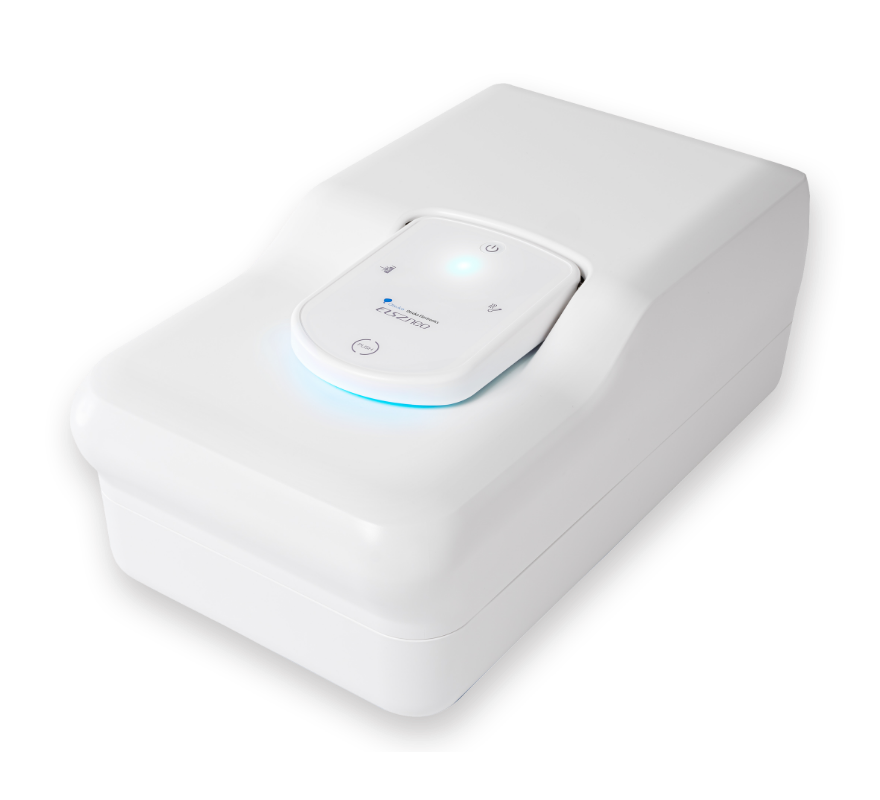
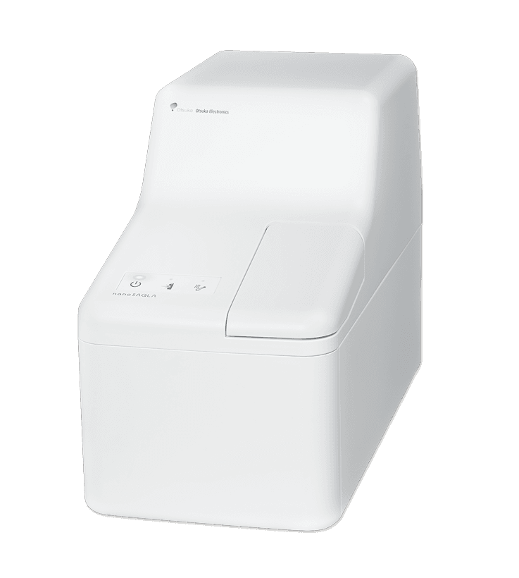
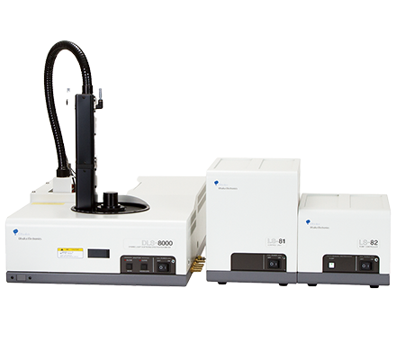
Our equipment (nanoSAQLA, ELSZ series) is based on the light scattering measurement technique. The systems are a particle size measuring instrument by dynamic light scattering method that measures the fluctuation of scattered light due to the Brownian motion of the particles, and a zeta potential measuring instrument by electrophoretic light scattering method that measures Doppler shift of scattered light while the particles are electrophoresed. They provide information on the dispersed state of fine particles in a solution.
With the dynamic light scattering method, it is possible to measure the particle size distribution in the nano and micron range from 0.6 nm to 10 μm. In addition, our instrument can measure not only the dispersion system of inorganic particles and organic particles but also a wide range of particles (colloids) with solution systems such as biological polymers and polymer electrolytes and provide information on dynamic changes such as the aggregation process of particles.
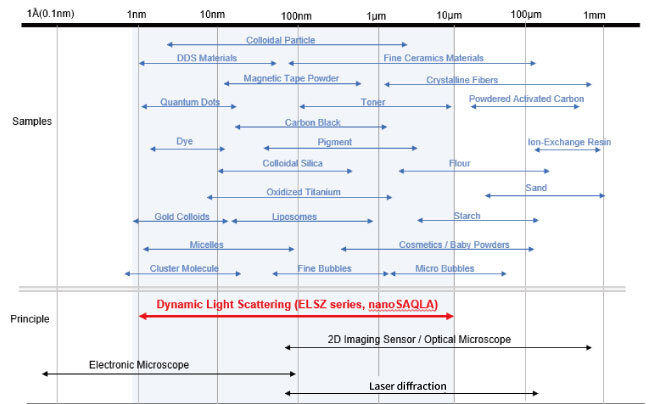 Figure 1. Particle size range and measurement method of various particles
Particle size measurement principle
As shown in Fig. 1, the particle size measurement range of our instruments by the light scattering method is 0.6 nm to 10 μm. Particles in this range change their position, orientation, and morphology from moment to moment due to Brownian motion such as translation and rotation in a solution. When these particles are irradiated with laser light and the scattered light emitted is detected, fluctuations of the scattering intensity depending on Brownian motion of the particles are observed. Therefore, by observing the temporal fluctuation of scattered light, the velocity (diffusion coefficient) of Brownian motion of the particle can be obtained, and the particle size can be estimated from them.
Our instruments uses this dynamic light scattering method to obtain the particle size distribution.
The following is a comparison of various particle size measurement methods.
Table 1. Comparison of various particle size measurement methods
| Measurement method | Measurement range of particle size(μm) | Measurement physical quantity | Advantages | Disadvantages |
|
Dynamic light scattering |
0.0006~10 |
Fluctuation of scattered light |
Capable of measuring particles smaller than sub-micron, No information of the particle required (Only refractive index and velocity of the solution required) |
Easily dependent on scattering intensity, Easily affected by dust |
|
Laser diffraction |
0.015~3000 |
Diffraction scattering pattem |
Simple, Wide measurement range |
Refractive index of the particle required, Low measurement accuracy for particles smaller than submicron, Particle size calculation differs depending on the model |
|
Centrifugal sedimentation method |
0.01~300 |
Amount of transmitted light |
Low cost, Simple |
The density and refractive index of the particle required, Long measurement time for submicron particles, Absorption coefficient correction required |
|
Field flow flactionation method |
0.01~1 |
Amount of transmitted light |
Capable of measuring particles smaller than submicron, High resolution |
The density and refractive index of the particle required |
|
Electrical sensing zone method (Coulter counter) |
0.1~1000 |
Current/Voltage |
Capable of measuring particle volume |
Narrow measurement range, Replacement of pore required, Difficult to measure unknown particle size |
Since laser diffraction method uses the light diffraction phenomenon and Mie scattering phenomenon to determine the particle size, it is possible to measure in a wide particle size range, but it requires the refractive index of the particles. Moreover, measurement accuracy decreases considerably in the submicron region because the angle dependence of Mie scattering is not substantially observed.
The centrifugal sedimentation light transmission method is easy to operate, but has the disadvantage that the smaller the particle size is (the smaller the difference in specific gravity between a sample and a dispersion medium), the longer the measurement time takes.
The FFF method can obtain a high-resolution particle size distribution, but it requires particle density and refractive index.
The electrical sensing zone method can measure the particle volume, but it is desired to expand the dynamic range.
As you can see, each of the various particle size measurement methods has its own characteristics, but it can be seen that only the dynamic light scattering method can measure particle size which the electron microscope can measure, thus it can be used for ultrafine particle measurement.
Note) Other measurement principles
- Laser diffraction method: The particle size is determined by using the diffraction phenomenon of light (Fraunhofer phenomenon) and the Mie scattering phenomenon.
- Centrifugal sedimentation light transmission method: The particle size is measured from the relationship between the particles size settling in the medium and the settling velocity.
- FFF method (Field Flow Fractionation): Particles are injected into a duct filled with a cleaning liquid, and when an external force field is applied to the duct, the particles are deposited on the duct according to the applied external force. When a laminar flow is applied to such deposited particles, the particles at a high flow velocity position are carried farther. The particles at that time are detected by the light transmission method to obtain the particle diameter.
- Electrical sensing zone method : Detects fluctuations in electrical resistance that occur when particles cross an electric circuit formed through pores in an electrolyte solution, and the volume and number of particles are determined.
■Particle size from Brownian motion
Fine particles dispersed in a suspension or a solution usually have Brownian motion, which is slower for larger particles and faster for smaller particles. (Figs.2 and 3)
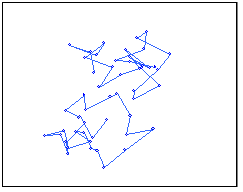 Figure 2. Brownian motion of small particles
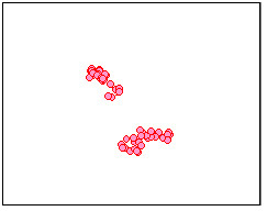 Figure 3. Brownian motion of large particles
The difference in Brownian motion due to the difference in particle size is observed as the difference in the rate at which the particles diffuse in a solution, as shown in Fig. 4. Therefore, the particle size can be obtained by measuring the diffusion coefficient.
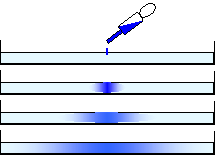 ○Small particles
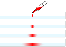 ○Large particles
Figure 4. A model showing the difference in diffusion rate between small particles (left)
and large particles (right)
When a sphere with a particle diameter d (diameter) is dispersed in a solvent having a viscosity η0, the relationship with the diffusion coefficient D is expressed by Stokes-Einstein equation as follows.
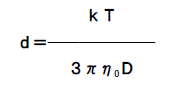
Here, k is the Boltzmann constant and T is the absolute temperature.
Principle of dynamic light scattering method
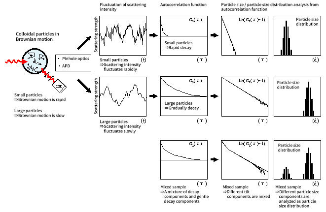
Fine particles dispersed in a suspension or a solution usually have Brownian motion, which is slower for larger particles and faster for smaller particles. At this time, when the particles that are in Brownian motion are irradiated with laser light, the fluctuation of the scattered light according to the speed of each Brownian motion is observed.
In the dynamic light scattering method, as shown in Fig. 5, the particles dispersed in a solution are irradiated with laser light, and the scattered light is observed by the photon detector. At this time, the scattered light from the particles interferes with each other as shown in Young's optical interference experimental model (Fig. 6). Furthermore, since the particles are constantly moving in position due to Brownian motion, the intensity distribution due to the interference of scattered light is also constantly fluctuating. Therefore, if a pinhole or optical fiber optical system is used, this Brownian motion can be observed as fluctuations in scattered light intensity.
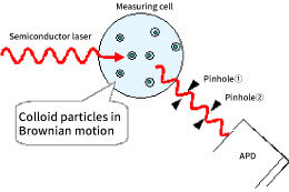 Figure 5. Schematic diagram of dynamic light scattering method
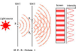 Figure 6. Young's optical interference experimental model
The observed chronological fluctuations of scattered light differ depending on the particle size, as shown in Fig. 7 and 8.
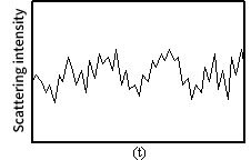 Figure 7. Fluctuation of scattered light of small particles
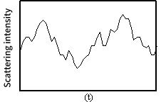 Figure 8. Fluctuations of scattered light of large particles
By observing this fluctuation, the autocorrelation function is obtained by the photon correlation method, and the cumulant method and the histogram method analysis are used to obtain diffusion coefficient indicating the Brownian motion velocity, and the particle size and particle size distribution.
The autocorrelation function is based on the scattering intensity I (t) at an arbitrary time (t), and the correlation for the scattering intensity I (t + τ) after (τ) time is expressed by the following equation.
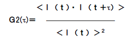
Here, <> represents the average. This autocorrelation function depends only on time (τ) and does not depend on measurement start time (t). In the autocorrelation function, when τ is small, the particles do not move much, so the change in the amount of scattered light is small and shows a high correlation, but when τ is large, the position of the particles becomes uncertain, so the amount of scattered light also changes randomly. The correlation is almost non-existent. Therefore, the resulting autocorrelation function is an exponential decay curve.
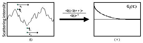 Figure 9. Scattered light intensity and autocorrelation function
The particles change their position by Brownian motion as shown in Fig.10. The autocorrelation function expresses the degree of particle overlap between τ1, τ2, τ3 ... from the position of particles at a certain reference time as a function of time. As a result, as shown in Fig. 11, the degree of overlap decreases with time, so the autocorrelation function G2 (τ) expresses a function that decays with time.
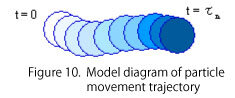
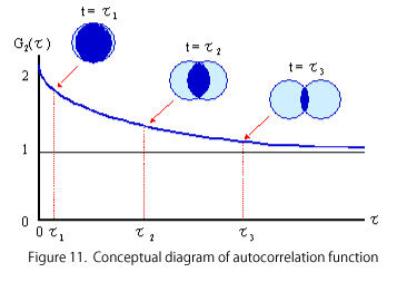 Figure 9. Scattered light intensity and autocorrelation function
Refer to the materials of the 12th Scattering Study Group "Dynamic Light Scattering-Basic Seminar" by Professor Mitsuhiro Shibayama, Tokyo University
Analyzing the variation of scattering intensity using the photon correlation method yields a correlation function with a short correlation time for small particles and a long correlation function for large particles. The correlation function contains information about the translational Brownian motion of suspended particles, and the particle size and particle size distribution can be obtained by a calculation formula.
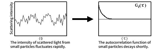 Figure 12. Fluctuations of scattered light from small particles and its autocorrelation function
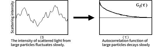 Figure 13. Fluctuations of scattered light from large particles and its autocorrelation function
Features of photon correlation method
Table 2 shows a comparison of the photon correlation methods. The photon correlation meter used in our instruments is a software method. Our dynamic light scattering photometer and zeta potential analyzer incorporate both the T.I. method and the T.D. method and are considered for accuracy in a wide range. The conventional T.I. method has good accuracy when the light is weak and the particle size is small, and the T.D. method enables high-precision measurement when the particle size is large, and the amount of light is large. Figure 14 shows each calculation method.
Table 2. Comparison of photon correlation methods
|
Photon Correlation Method |
Advantages |
Disadvantages |
|
|
Software method (The number of photons counted by the hardware is stored in the memory, and the correlation function is obtained by adding, subtracting, and multiplying by the software (CPU).) |
Time interval method |
To see the change in the number of clocks between photon pulses, sampling time can be reduced, time resolution and distribution accuracy are good |
Difficult to deal with large particles and long correlation. |
|
Time domain method |
Since the change in the number of photon pulses during the sampling time is observed, it is easy to deal with long correlations, and the accuracy of large particles is high. |
The measurement efficiency decreases when the amount of light is weak. |
|
|
Hardware method (counts the number of photons at a predetermined gate and calculates the correlation function by adding, subtracting, and multiplying electrically (shift register)) |
Shift register method |
Output of the correlation function in real time is possible (correlation time = measurement time) ) Short dead time (50nsec) |
Accuracy is reduced when the amount of light is large or weak. The function is fixed due to the hardware configuration, The number of data channels is small, Impossible to retain an irregular data removal (dust cut) function due to dust |
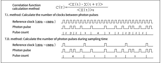 Figure 14. Calculation method of T.I. method and T.D. method
The nanoSAQLA and ELSZ series are based on the TD method and employ a new correlation meter that covers the disadvantages of both the conventional TI and TD methods. The features are described below.
- Covers correlation time of 1 μsec to 1 sec with one measurement
(measurement conditions are the same) - Calculates particle size at 2-second intervals
- Maintains dust cut function
- Measurement efficiency (ratio of data acquisition time to measurement time) is achieved nearly 100% ( High-precision measurement in a short time)
In this way, the new correlation meter can ensure the same or better accuracy than the two conventional methods.
Analysis principle of dynamic light scattering method
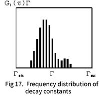
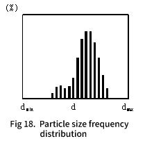
From the autocorrelation function obtained by the photon correlation method, the average particle size d (hydrodynamic diameter) and polydispersity index are obtained by the cumulant method, and the particle size distribution is obtained by the histogram method.
| ●Autocorrelation function The intensity autocorrelation function G2 (τ) obtained directly from the temporal change of scattering intensity is expressed by the following equation.  When the particles are monodispersed, G1 (τ) is a single exponential decay curve and is expressed as follows using the decay constant Γ. 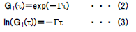 Γ is expressed as follows using the translational diffusion coefficient D. 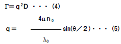 q: Scattering vector, n0: Refractive index of solvent, λ0: Wavelength of laser light ●Stokes-Einstein equation Using the Stokes-Einstein equation, the particle size (Stokes diameter) can be obtained from the diffusion coefficient. 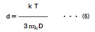 d: Particle diameter (hydrodynamic diameter), k: Boltzmann constant, T: Absolute temperature, η: Viscosity of solvent ●Cumulant method analysis The average particle size and dispersity index are obtained from the first and second order coefficients, respectively by the series expansion of cumulant generating function. 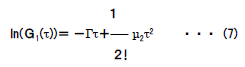 The cumulant average particle size is obtained from Γ. The polydispersity index is obtained by normalizing μ2 by the square ofΓ (μ2 / Γ2) and indicates the degree of polydispersity of the particle size distribution. ●Histogram analysis In the histogram method, the distribution is represented by a finite number of Γj and approximated using the nonlinear least squares method. 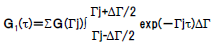 Each attenuation constant is converted into a particle size using equations (4) and (6). The particle size distribution can be obtained by displaying a histogram with this as the horizontal axis and the frequency obtained here as the vertical axis. |
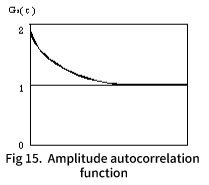 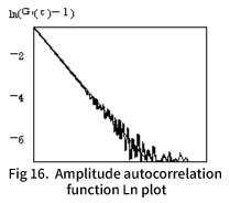   |
[Outline of dynamic light scattering method]
Features of dynamic light scattering software
It is equipped with a soft correlator that can measure under the optimum measurement conditions according to the sample. In addition, the software has excellent operability.
- Highly accurate data acquisition is possible by the photon correlation method.
- Highly reliable data can be obtained by abundant analysis modes.
- Measurement is possible in a short time.
- Measurement conditions can be set automatically.
- The temporal change of particle size can be measured.
- Overlapping display of particle size distribution is possible.
Particle size measurement and its application
Particle size measurement by dynamic light scattering is used for the following purposes. Application fields and application examples of our equipment are also shown in the table.
Table 3. Application fields and application examples
|
Pigments, inks and toners |
dispersion / aggregation / stability index, particle size / particle size distribution management |
|
Semiconductor Polishing (CMP) Particles |
dispersion / stability evaluation, particle size / particle size distribution management |
|
Latex |
calibration of standard particles, quality control of mixing ratio,judgment of the effect of surface modification, latex aggregation monitor |
| Emulsions | stabilization index, evaluation of emulsification conditions |
| Ceramics | index of micronization, index of dispersibility, evaluation of dispersant |
| Inorganic sol Magnetic material |
indicators of primary and secondary particles and aggregation/stability |
| Ultrafine particles | examination of manufacturing method. Stability indicator |
| Particle composite (Surface modification) |
indicator of aggregation / stability |
Table.4. Field and Applications-
|
Field |
Applications |
|
Polymer / chemical industry |
standard latex, industrial latex, paint emulsion, adhesive emulsion, fluorescent particles, magnetic particles, metal colloids, petroleum related, detergents, waxes, surfactants |
|
Ceramics / color materials industry |
pigments, inks, carbon black, ceramics, inorganic sol gels, cement, photocatalytic materials (titanium oxide fine particles), photosensitive materials (silver halide) |
|
Semiconductor / Display |
semiconductor polishing particles, CMP particles, antireflection film material, phosphor fine particles, photosensitive resin |
| Biotechnology/ Pharmaceutical industry | medical emulsion, cosmetic emulsion, DDS particles, liposomes, polymer micelles, surfactant micelles, diagnostic latex, iagnostic gold colloid, fat emulsion protein, virus |
| Food industry | food emulsions, fragrance emulsions, milk, dairy products, beverages, emulsifiers |
| Environmental chemistry | agricultural emulsion, carbon black, carbon sludge |
(Revised in September, 2022)